Stochastic Optimal Control with Terminal Constraints

Stochastic Optimal Control with Terminal Constraints

Yuan,Shi

PhD Mathematics, Imperial College London

Abstract: The authors study a few constrained Stochastic Optimal Control Problems with terminal constraints, such as Linear Quadratic Mean-Field problem or Non-Markovian problem with stochastic coefficients. The authors draw equivalence relationship between the Fritz John condition and Karush–Kuhn–Tucker (KKT) conditions. Then they construct an unconstrained problem with the Lagrange Multiplier derived from Fritz John condition. Finally, they show the equivalence between the optimality of the unconstrained problem and its original problem.

Keywords: Duality, Lagrange Multiplier, Fritz John Condition, KKT conditions, Linear Quadratic Mean-Field Control, Mean-Field Forward Backward Equations (MF-FBSDEs)

1Introduction

Constrained Stochastic Optimal Control has always been a popular area of study. Different methods are used to tackle different constraints. Such as duality [7], HamiltonJacobi-Bellman (HJB) [3, 2], and most naturally Lagrange multiplier methods. Flam [5] gave a proof of necessary conditions of KKT in terms of subdifferential for discrete Markovian problem followed by a correction in [6]. Since then, more people have used the Lagrange multiplier method to convert a constrained problem into an unconstrained one and apply the established method to solve problems, such as those in [11, 1, 9]. While many of the results can be applied to more general problems, which are nonconvex and non-Frechet differentiable, they often complicate the problem. Moreover, due to generality, the local extrema obtained using KKT are often not global extrema. As such, inspired by the Fritz John condition mentioned in [4], which does not contain any requirement on the differentiability of the problem, we generalised the results there from discrete problems into continuous time problems and draw relationships between the FJ condition and KKT conditions, the later of which can be shown to be necessary and sufficient to the optimality of original problem under nice enough conditions.

In this section, we studied two problem. The first one is inspired by problem in [12], which is linear quadratic, containing stochastic coefficients and convex cone constrained control. When the terminal constraint also follows a similar quadratic form, the unconstrained problem can be solved using the same method proposed in the paper and hence give an optimal solution to the original constrained problem. The second problem is inspired by [15], which is mean-field.

2Lagrange Multiplier for Stochastic Optimal Control Problem with additional terminal inequality constraints

Let T > 0 be a fixed terminal time, {Wt,t ∈ [0,T]} a RN-valued standard Brownian Motion with entries Wm,m = 1,2...N, on a complete probability space (Ω,F,P).

Lemma 2.1 L2F(0,T;RN) forms a Hilbert space with inner product ⟨x,y⟩ defined as

.

Lemma 2.2 Every bounded sequence in Hilbert space has a weakly convergent subsequence.

Proof. For example refer to [8].

Theorem 2.3 (Banach Sak’s Thoerem) In a uniformly convex Banach space, any weakly converging sequence has a subsequence whose Cesaros-mean converges strongly, where the Cesaros-mean denotes the arithmetic mean.

Proof. For example refer to [10].

Assume that r,Q ∈ L1F(0,T;R), θ,S ∈ L1F([0,T],RN), σ,R ∈ L1F(0,T;RN×N) are uniformly bounded. For all (z,ω,t) ∈ RN × Ω × [0,T], there exists a constant k > 0 such that

z⊺σ(ω,t)σ⊺(ω,t)z ≥ k|z|2,

R symmetric and the matrix is positive definite for almost all (ω,t) ∈

Ω × [0,T].

Lemma 2.4 (Schur’s Complement)

Proof. For example, refer to Section 1.4 Theorem 1.12 from [16].

Lemma 2.5 (Fatou’s Lemma) Given a measure space (Ω,F,µ) and a set X ∈ F, let {fn} be a sequence of (F,B)-measurable non-negative functions fn : X → [0,+∞]. Define the function f : X → [0,+∞] by setting f(x) = liminfn→∞ fn(x), for every x ∈ X. Then f is (F,B)-measurable, and also , where the integrals may be infinite.

Proof. This is a direct application of Monotonic Convergence Theorem. Refer to Theorem 2 from section 5.2 in [14].             

Theorem 2.6

(Jensen’s Inequality) Let (Ω,F,P) be a probability space, X an integrable real-valued random variable and f a convex function. Then:

f(E[X]) ≤ E[f(X)].

Proof. Refer to [13] for a general proof on an infinite-dimensional space.

Let a,c,m,n,k be bounded variables valued in R with a,m being positive. Under the quadratic and convex setting, for x ∈ R,π ∈ RN, let

Then for the state process Xπ ∈ L2F(0,T;RN) and control π ∈ L2F (0,T;RN), the optimization problem is as the following:

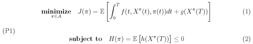
where dXπ(t) = (r(t)Xπ(t) + π⊺(t)σ(t)θ(t))dt + π⊺(t)σ(t)dWt; Xπ(0) = x0(3)

and

A:= {π ∈ L2F(0,T;RN) : π(t) ∈ K for all t ∈ [0,T] a.e.},

with K RN a closed convex set containing 0.

Define

B:= {π ∈ A : H(π) ≤ 0}.

We call π admissible if it is in B and the pair (π,Xπ) is called admissible if Xπ is a strong solution to (3). Let V (x0) denote the value function of (P1), i.e. V (x0) = infπ∈B J(π). Lemma 2.7 B is convex.

Proof. B = A ∩ {π : H(π) ≤ 0} and if it can be shown that B is a union of 2 convex sets, then it is also convex. It is straightforward to see that A is convex. To see that {π : H(π) ≤ 0} is convex, first observe (3) is linear about π and X. Therefore Xπ˜ = Xµπ1+(1−µ)π2 = Xµπ1 + X(1−µ)π2 = µXπ1 + (1 − µ)Xπ2 for µ ∈ [0,1] and (πi,Xπi) admissible. Given h convex, we can conclude that

.

Hence π˜∈ {π : H(π) ≤ 0} and so B is convex.

If the solution to the non-constrained problem (1) already satisfies the constraint (2), then we are done here. Thus it is advisable to solve the problem without additional constraint first.

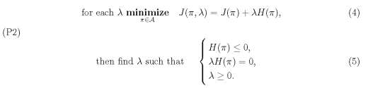
For a more general solution, let’s introduce a Langrange Multiplier λ ≥ 0 to reduce constrained problem (P1) to an unconstrained case:

While we can also draw equivalent relationship between Karush–Kuhn–Tucker conditions and the Fritz John condition similar to the deterministic optimal control, in stochastic case, we shall use an alternative version of the Fritz John (FJ) condition mentioned in [4].

Define

C := {(r,s) ∈ R × R : J(π) ≤ V (x0) + r,H(π) ≤ s, for some π ∈ A}.

Then the following assumption ensures that we will arrive at FJ condition:

(FJ1) The convex hull of C, ConvC has non-empty interior and (0,0) lies on the boundary of ConvC.

Lemma 2.8 C is convex.

Proof. Suppose (r1,s1),(r2,s2) ∈ C, so there exists π1,π2 ∈ A s.t.

J(πi) ≤ V (x0) + ri,H(πi) ≤ si, for i ∈ {1,2}.

Then for any real number µ ∈ [0,1], π˜= µπ1 + (1 − µ)π2, r˜= µr1 + (1 − µ)r2 and s˜ = µs1 + (1 − µ)s2,

J(π˜) ≤ µJ(π1)+(1−µ)J(π2) ≤ µV (x0)+µr1 +(1−µ)V (x0)+(1−µ)r2 ≤ V (x0)+r,˜

H(π˜) ≤ µH(π1) + (1 − µ)H(π2) ≤ µs1 + (1 − µ)s2 ≤ s.˜ Hence π˜∈ C and C is convex.             

Also, as long as is non-empty so it only suffices to assume the origin is on the boundary. As such assumption (FJ1) is equivalent to the following condition under the current problem setting:

and origin is on the boundary of C.

Theorem 2.9 (Fritz John Condition) With (FJ2) satisfied, one can find a non-zero pair (r∗,s∗) ∈ R≥0 × R≥0 such that

r∗V (x0) = inf π∈A{r∗J(π) + s∗H(π)}.(6)

Proof. From (FJ2), the origin is on the boundary of C, as such, we can find a supporting hyperplane to the convex hull through the origin. Hence there exists a non-zero pair (r∗,s∗) ∈ R×R such that r∗r+s∗s ≥ 0, for any (r,s) in C. If r∗ < 0, for any pair (r,s) we can pick arbitrarily large r˜such that (r˜,s) is still in C. So there exits r˜such that r∗ r˜+ s∗s < 0 which contradicts the result. Hence r∗ ≥ 0. With a similar argument, s∗ ≥ 0. Furthermore, by definition of C, for any π ∈ A, (J(π) − V (x0),H(π)) ∈ C and

r∗(J(π) − V (x0)) + s∗H(π) ≥ 0.

Hence

r∗V (x0) ≤ infπ∈A {r∗J(π) + s∗H(π)}.

The reverse is trivially true since s∗ ≥ 0 and H(π) ≤ 0 for any π ∈ B. Then,

.

Hence,

.

To ensure the existence of the Lagrange multiplier, another assumption has to be made: (SF1) There exists π ∈ A s.t. H(π) < 0.

Theorem 2.10 If both (FJ2) and (SF1) are satisfied, then we can always find a Lagrange multiplier λ such that

.

Proof. Suppose for a contradiction for all pair (r∗,s∗) ∈ C, r∗ = 0, then by non-zeroness,

s∗ > 0, together with (SF1)

,

which leads to a contradiction. Hence we can find such r∗ > 0. pide r∗ on both sides of (6) to obtain

.

We can conclude   as the non-negative Lagrange multiplier.

Next, we want to show the Lagrange multiplier indeed satisfies (5).

Theorem 2.11 Under (FJ2) and (SF1), we can find λ such that

V (x0) = inf π∈A{J(π) + λH(π)}

and (5) is true.

Proof. From Theorem 2.10, we can find a non-negative Lagrange multiplier λ s.t.

.

As λ ≥ 0, for any π ∈ B, J(π) + λH(π) ≤ J(π), so

V (x0) ≤ inf π∈B{J(π) + λH(π)} ≤ inf π∈BJ(π) = V (x0).

Hence infπ∈B{J(π) + λH(π)} = infπ∈BJ(π) = V (x0).(7)

Then, by the definition of infimum, we can find a sequence {πn} s.t. πn ∈ A, H(πn) ≤ 0 and

.

By completing the square in the running cost

.

From Lemma 2.4, Q > 0 and R − SQ−1S⊺ ≻ 0. By the Min-Max Theorem,

. Hence, .

The terminal cost is quadratic with quadratic coefficient (a + λm) > 0. Therefore, it is bounded from below by some number κ. Then .

As ), a bounded sequence in the Hilbert space L2F(0,T;RN). By Lemma 2.2, there exists a weakly convergent subsequence {πi,i ∈ I1}. The by Thoerem 2.3, we can again find a subsequence {πi,i ∈ I2 I1} such that, after reordering the subsequence, the Cesaro-mean converges strongly to π˜, i.e.

.

As L2F(0,T;RN) is a Hilbert space, the closed subset of Hilbert space is complete, hence the limit π˜∈ B.

Additionally note J(π) is convex and bounded from below, then by Fatou’s Lemma 2.5 and Jensen’s inequality 2.6:

Substitute π˜to (7) we have J(π˜) = infπ∈B{J(π) + λH(π)} ≤ J(π˜) + λH(π˜) ≤ J(π˜)

Therefore, λH(π˜) = 0.

On the other hand, for sufficiency,

Theorem 2.12 Suppose that there exists a pair (π∗,λ∗) that solves (P2). Then the value function to (4), J(π∗,λ∗) equals the value function of (P1). Furthermore, the corresponding (Xπ∗,π∗) is optimal to the original constrained problem (P1), that is

J(π∗,λ∗) = J(π∗) = V (x0).

Proof. As (π∗,λ∗) is optimal to the unconstrained problem (P2), for any π ∈ B, we have

J(π,λ∗) ≥ J(π∗,λ∗).

From (4) and (5),

J(π) + λ∗H(

π) = J(π,λ∗) ≥ J(π∗,λ∗) = J(π∗) + λ∗H(π∗) = J(π∗).

Therefore, for any π ∈ B,

J(π) = J(π∗) − λ∗H(π) ≥ J(π∗),

that is

.

Hence we can show that

J(π∗,λ∗) = J(π∗) = V (x0).

Corollary 2.13 Under the same setting as in Theorem 2.12 above, we can find a nonzero pair (r∗,s∗) ∈ R≥0 × R≥0 satisfy (6).

Proof. The proof is straight forward from results of Theorem 2.12.

.

Time both sides by some positive number to arrive at (6).

Therefore, we have shown that under (FJ2) and (SF1), the FJ condition is equivalent to the KKT conditions. Furthermore, Theorem 2.11 shows that with an optimal solution to the constrained problem (P1), there exists an optimal pair of control and Lagrange multiplier to solve the unconstrained problem (P2) while Theorem 2.12 shows that the KKT conditions are sufficient for the optimal solution to the non-constrained problem (P2) to match the optimal solution to the constrained problem (P1). As such, we have built the necessary and sufficient conditions between the optimality of constrained and unconstrained problems. Lastly, it is natural to ask what would happen when (FJ2) and (SF1) are not satisfied.

Lemma 2.14 If (0,0) ∈ C, then it will be on the boundary.

Proof. Suppose for a contradiction, then the origin will be in the interior of C which means we can find ε > 0 such that the ball B((0,0),ε) C. Hence we can pick (µ,0) ∈ C where −ε < µ < 0 which by definition of C says there exists a π ∈ A such that J(π) ≤ V (x0) + µ < V (x0) contradicting the fact V (x0) is the infimum.

Therefore, if (FJ2) is not satisfied, either , which is a trivial case, or (0,0) not in C.

Lemma 2.15 If C is not empty, then (0,0) ∈ C.

Proof. Suppose for a contradiction, if (0,0) not in C, then there exists ε > 0 such that B((0,0),ε) Cc, the complement of C. So for all π ∈ A and (r,s) ∈ B((0,0),ε), J(π) > V (x0) + r or H(π) > s. Pick r,s > 0, then for all π ∈ B, J(π) > V (x0) + r which means V (x0) = infπ∈B J(π) ≥ V (x0)+r > V (x0), leading to a contradiction.

Lemma 2.16

If (SF1) is not satisfied, then the constrained problem is equivalent to (1) subject to H(π) = 0.

Proof. If (SF1) is not satisfied, then for any π ∈ B, H(π) ≥ 0. Combining with the constraint (2), the new constraint would be H(π) = 0.

Remark Although Theorem 2.12 says that the optimal control for the unconstrained problem matches that of the constrained problem, we still need a way to find the optimal control and optimal value. The steps are to first fix a Lagrange multiplier λ, then solve

(4), for example, using the established method in [12]. Define

as an alternative version of (3) without the constant term. Then, for any fixed λ ≥ 0, J(π) + λH˜(π) can be treated as the cost function in [12] and solved accordingly.

Subsequently, pick λ∗ that satisfies (5) which definitely exists by Theorem 2.11.

3Lagrange Multiplier for Mean-Field Stochastic Optimal Control Problem with additional terminal inequality constraints

In the section we change the setting to a mean-field problem. Most of the proofs will be similar to 2, so they will be omitted. However, because most of the studies on meanfield stochastic optimal control, especially linear-quadratic, center around deterministic coefficients, we will use new settings similar to those in [15]:

(H1) A,A¯ ∈ L1(0,T;Rn×n), B,B¯ ∈ L2(0,T;Rn×m), C,C¯ ∈ L2(0,T;Rn×n) and D,D¯ ∈ L∞(0,T; Rn×m).

(H2) Q,Q¯ ∈ L1(0,T;Sn),S,S¯ ∈ L2(0,T;Rm×n), R,R¯ ∈ L∞(0,T;Sm), GT ,G¯T ∈ Sn and gT ,g¯T ∈ Rn.

Let u ∈ U[t,T] := L2F(t,T;Rm) and the initial pair (t,ξ) from

D := {(t,ξ) : t ∈ [0,T],ξ ∈ LF2t(Rn)}.

Define the state process as

and the objective cost function being

(H3) There exists a constant δ > 0 such that

.

As (H1), (H2) and (H3) are the same as (A1), (A2) and (A4) from section 3 in [15],(8) admits a unique Xu ∈ L2F(C(t,T;Rn)) and the problem

minimizeJ(t,ξ;u)(8)

u∈U[t,T]

has a unique solution u∗ ∈ U[t,T] for each pair (t,ξ) ∈ D.

Additionally, it is also pointed out that (H3) is equivalent to J(t,ξ;u) being uniformly (strongly) convex.

Extending from Yong and Sun’s work, suppose there is an additional constraint at the terminal time,

,

where HT and while hT , h¯T and c are constant. Then the constrained problem will be

minimizeJ(t,ξ;u)

u∈U[t,T]

(P3)

subject toH(u) ≤ 0

Let U˜[t,T] = {u ∈ U[t,T] : H(u) ≤ 0} and V (t,ξ) denotes the value function so

V (t,ξ) := inf u∈U˜[t,T]J(t,ξ;u).

Similarly to Section 2, introduce the Lagrange multiplier and construct an unconstrained problem. Define J(t,ξ;u,λ) = J(t,ξ;u) + λH(u) then for each λ, the unconstrained problem becomes

(9)

Let its value function be V (t,ξ;λ), so

.

The KKT condition is finding λ such that

(10)

Define

C := {(r,s) ∈ R2 : J(t,ξ;u) ≤ V (t,ξ) + r,H(u) ≤ s, for some u ∈ U [t,T]}, and the assumption about C will be still be (FJ1).

Lemma 3.1 C is convex.

Proof. Since J is convex and the SDE (8) is linear, the proof is the same as in 2.8.

Assuming , we can again simplify (FJ1) to

and the origin is on the boundary of C.

Theorem 3.2 With (FJ3) satisfied, one can find a non-zero pair (r∗,s∗) ∈ R≥0 × R≥0 such that

.

Proof. The proof is the same as Theorem 2.9.

The strict feasibility says

(SF2) There exists u ∈ U s.t. H(u) < 0.

Theorem 3.3 If both (FJ3) and (SF2) are satisfied, then we can always find a Lagrange multiplier λ such that

.

Proof. Proof same as Theorem 2.10.

Theorem 3.4 Under (FJ3) and (SF2), we can find λ such that

and (10) is true.

Proof. According to (3.3.3) from [15], for each pair (t,ξ) ∈ D, J(t,ξ;u) can be expressed as quadratic equation on u and strictly convex from (H3). Hence it is bounded from below by for some α > 0 and κ ∈ R. Also U[t,T] is a Hilbert space so the proof will be the same as that in Theorem 2.11.

Theorem 3.5 For any pair (t,ξ) ∈ D, suppose that there exists a pair (u∗,λ∗) that solves (9) and satisfies (10). Then the value function J(t,ξ;u∗,λ∗) equals the value function of (P3). Furthermore, the corresponding (Xu∗,u∗) is optimal to the original constrained problem (P3), that is

V (t,ξ;λ∗) = J(t,ξ;u∗,λ∗) = J(t,ξ;u∗) = V (t,ξ).

Proof. The proof is the same as Theorem 2.12.

Remark For each λ, we can treat the unconstrained problem (9) as an example in [15] to solve. Then find λ

∗ that satisfies (10).

4Conclusion

Notice that most of the proofs only require finiteness of the value function and convexity of the problem. As such it is possible to apply the results to a more general settings, for example, the cost functions do not have to be limited to quadratic. Any convex function bounded below can be used instead.

Lemma 2.16 points out what would happen if the Strict Feasiblity condition is violated. The additional constraint H(π) would only be zero, and the problem becomes finding an optimal solution with the equality constraint, given that the additional constraint is always non-negative. Although the problem becomes limited, it would still be interesting to see what the solution would look like.

References

[1]T. R. Bielecki, H. Jin, S. R. Pliska, and X. Y. Zhou, Continuous-time mean-variance portfolio selection with bankruptcy prohibition, Mathematical Finance, 15 (2005), pp. 213–244.

[2]B. Bouchard, R. Elie, and C. Imbert, Optimal control under stochastic target constraints, SIAM Journal on Control and Optimization, 48 (2010), pp. 3501–3531.

[3]I. Capuzzo-Dolcetta and P.-L. Lions, Hamilton-jacobi equations with state constraints, Transactions of the American Mathematical Society., 318 (1990-01-01).

[4]I. Evstigneev and S. D. Fl˚am, Encyclopedia of Optimization, Springer US,

Boston, MA, 2009, ch. Stochastic Programming: Nonanticipativity and Lagrange Multipliers, pp. 3783–3789.

[5]S. D. Fl˚am, Lagrange multipliers in stochastic programming, SIAM Journal on Control and Optimization, 30 (1992), pp. 1–10.

[6]S. D. Fl˚am, Corrigendum: Lagrange multipliers in stochastic programming, SIAM Journal on Control and Optimization, 33 (1995), pp. 667–671.

[7]S. Ji and X. Y. Zhou, A maximum principle for stochastic optimal control with terminal state constraints, and its applications, Communications in Information & Systems, 6 (2006), pp. 321–338.

[8]J. Jost, Hilbert Spaces. Weak Convergence, Springer Berlin Heidelberg, Berlin, Heidelberg, 1998, pp. 271–280.

[9]A. Jourani and F. J. Silva,

Existence of lagrange multipliers under gˆateaux differentiable data with applications to stochastic optimal control problems, SIAM Journal on Optimization, 30 (2020), pp. 319–348.

[10]S. Kakutani, Weak convergence in uniformly convex banach spaces, tˆohuku math, J, 45 (1938), pp. 188–193.

[11]N. E. Karoui, S. Peng, and M. C. Quenez, A dynamic maximum principle for the optimization of recursive utilities under constraints, The Annals of Applied Probability, 11 (2001), pp. 664 – 693.

[12]Y. Li and H. Zheng, Constrained quadratic risk minimization via forward and backward stochastic differential equations, SIAM Journal on Control and Optimization, 56 (2018), pp. 1130 –– 1153.

[13]M. D. Perlman, Jensen’s inequality for a convex vector-valued function on an infinite-dimensional space, Journal of Multivariate Analysis, 4 (1974), pp. 52–65.

[14]A. J. Weir, Lebesgue Integration and Measure, Cambridge University Press, 1973.

[15]J. Yong and J. Sun, Stochastic Linear-Quadratic Optimal Control Theory: Differential Games and Mean-Field Problems, Springer International Publishing, 1 ed., 2020.

[16]F. Zhang, Schur complement and its applications, Springer New York, 2005.

1